 Summer… sun… swimming pool. Grab your drink, sit back and relax. Thinking back to yesterday’s family gathering, you might wonder whether the filtration system has done its job yet. Is the bright, sugary sports drink your nephew spilled in the pool really gone, or is it still there feeding unseen bacteria? Some might just add more chlorine to the pool, but a spectroscopist would want to find out.
And so we found ourselves wondering whether an Ocean Optics spectrometer would be sensitive enough for the job. Could a Flame spectrometer detect that diluted sports drink, or would the cooled detector of the QE spectrometer be needed to achieve the required limit of detection (LOD)? We resolved to put several spectrometers to the test to find out, but first we needed to think about noise.
“Noise” is Not Loud Music
When your car radio loses the station in a tunnel, you hear noise: a random, undesirable, signal completely lacking in information or structure. Noise is also present in the electric signal acquired by a spectrometer, and it is no less annoying to the spectroscopist. Spectrometer noise is caused by mechanical vibrations or environmental electrical fields, for example, from AC power lines. Good mechanical and electrical design principles can drastically reduce these effects.
Thermal noise
Unavoidable is the thermal, random motion of the electrons in the detector, which leads to signals that are not caused by light, often referred to as the “dark” signal. The dark signal is usually determined in a separate measurement without a light source, but due to its random nature this dark signal introduces noise in the spectrum. While the dark spectrum is generally subtracted from spectra prior to further analysis, its variability introduces some uncertainty into each measurement. In CCD-type detectors such as are used in our Flame-S, Maya2000 Pro, or QE Pro series spectrometers, a temperature change of just 7 °C cuts thermal noise in half; thermoelectrically cooling the detector (as in the QE Pro spectrometer) dramatically reduces the dark signal and the associated noise to allow the detection of very low light levels.
Thermal noise is especially important in near-infrared detectors, which are designed to detect low-energy photons (corresponding to wavelengths beyond what the eye can see). Very little energy is required of the photons to produce a signal in an IR detector, and thus thermal energy has an equally easy time generating a “dark” signal. The energy threshold for introducing thermal noise drops dramatically as the wavelength being recorded gets longer. In contrast to CCD detectors, however, the dark signal from near infrared detectors is very reproducible and can easily and precisely be subtracted. Furthermore, cooling the detector can reduce the dark signal significantly.
Counting Noise
Deep down, CCD-type detectors count the number of electrons that were kicked out of a “well” (the pixel) by the incoming photons. Depending on its “depth,” the maximum number of electrons that fit into a single well varies between less than 100,000 (Flame-S detector) to over one million (QE Pro detector). Due to the statistical nature of this counting process the exact number of electrons detected varies from measurement to measurement (even for a perfectly constant light level) with a standard deviation equal to the square root of the number of the electrons required to fill the well. The detector in the Flame-S, for example, with a well depth of approximately 62,500 electrons per pixel, produces a counting noise with a standard deviation of 250 electrons.
However, we can use the same laws of statistics to help to reduce this counting noise by averaging over repeat measurements. In OceanView software, this corresponds to the setting in “Scans to Average.” The noise level will decrease by the square root of the number of averages chosen, as shown in Figure 1, in which use of 100 averages leads to a ten-fold decrease in noise. Keep in mind, though, that using a large number of averages will increase the update time between spectra proportionally. This may be unsuitable for observing rapidly changing phenomena. Also, very long measurement times can be affected by slow drifts such as the light source output or temperature changes in the spectrometer. Thus, the number of averages chosen must balance the need for reduced noise with the type of sample being measured and the environment in which it is measured.
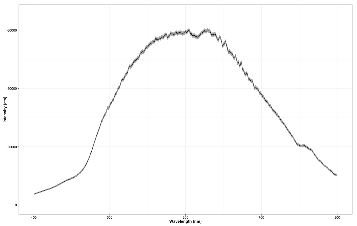
Figure 1: Effect of signal averaging on the noise level for a halogen lamp spectrum in a Flame-S spectrometer. The grey band indicates the fluctuations of individual spectra, the black line their average. The width of the grey band becomes narrower as more spectra are averaged in the acquisition.
Pixel to Pixel Variations
Neighboring pixels in photodiode array spectrometers are usually illuminated with comparable light levels and should therefore produce similar signals. Counting noise, as explained above, can lead to differences in the recorded signal for neighboring pixels and give the appearance of a “noisy” spectrum. However, not every pixel-to-pixel variation in the signal is caused by noise. For example, the dark signal for every pixel of a near-infrared InGaAs detector (such as in the Flame-NIR spectrometer) is different, and might give the appearance of a “noisy” spectrum, but as this signal is very reproducible from measurement to measurement, it is not noise and cancels upon dark subtraction.
As most spectrometers “oversample” the spectrum (that is, the optical resolution exceeds the distance between two pixels on the detector), one can average the signal from several neighboring pixels to decrease noise without losing spectral resolution. In OceanView this type of noise reduction is performed through boxcar averaging. The number of pixels included in the average on either side of the center pixel is selected with the “Boxcar width” setting, with zero corresponding to no averaging.
Pixels averaged = 2*Boxcar width + 1
However, once the total number of pixels included in the average exceeds the pixel resolution of the spectrometer, one starts to trade off smoothing against spectral resolution. The pixel resolution of the spectrometer is dependent on the spectrometer bench and slit size. For a Flame-S spectrometer with a 10 µm slit, for example, a boxcar width of 2 or more will begin to degrade the resolution of the spectrometer. This is often not an issue, but should be considered for applications requiring high resolution, or in which there are sharp features prone to detector saturation, like the D-alpha line observed in a deuterium lamp spectrum.
If the number of pixels averaged exceeds the pixel resolution of the spectrometer, the smoothed resolution of the spectrometer can simply be calculated by using the number of pixels averaged in place of the pixel resolution. Figure 2 illustrates the effect of boxcar averaging on the appearance of a lamp spectrum.
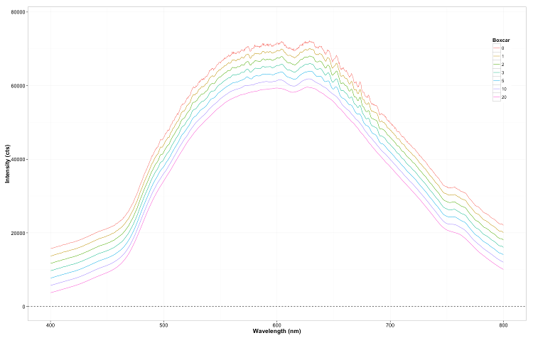
Figure 2: Effect of boxcar averaging on a halogen lamp spectrum as measured by a Flame-S spectrometer. The spectra are offset for clarity. Note that increasing the boxcar width reduces the noise, but will also wash out spectral features at higher boxcar width values.
Signal to Noise Ratio (SNR, or S:N)
The most critical parameter for a high-quality spectrum is the ratio of the signal level to the noise level; taking every step to minimize the noise does not do any good if the signal itself is equally small. On the flip side, even though Ocean Optics’ STS spectrometer tends to yield smaller signals than other spectrometer lines, its detector’s noise level is extraordinarily low, leading to one of the best signal-to-noise ratios in the product portfolio.
In addition to the noise reduction approaches discussed above, increasing the signal level will also improve the signal-to-noise ratio and hence the measurement quality. In general, one should strive to use the full dynamic range of the detector, as the signal to noise ratio increases with the square root of the number of signal counts. Several avenues are possible to achieve this goal:
Increase the light source output
Switch to a larger diameter for the fiber transferring the light to the sample to capture more light from the source
Increase the integration time of the detector
Limit the incoming lamp spectrum to just the wavelength span of interest to use the full dynamic range of the detector in the region where it matters most. This is especially true for the edges of the spectrum, which often suffer from lower intensities.
Conclusion
Reducing noise and increasing signal-to-noise are essential steps needed to detect the smallest concentration levels of an analyte of interest, like your nephew’s sports drink in the swimming pool. In this discussion of noise, we’ve learned that it is good to keep boxcar width fairly low (or at least to ensure that it does not smooth out spectral features you may need), and to set averages high (but not too high or you’ll be waiting all day for your spectrum!). We also discovered that noise, signal, and signal to noise ratio vary from one spectrometer to another, and that system design and software settings can help to maximize this ratio.


")


