How to Display Subranges across a Spectrum in OceanView Software

Using the OceanView Schematic Function to Customize Your Project

OceanView is the flagship software program for Ocean Optics spectrometers. Beyond simple data visualization, OceanView allows users to generate, customize and save spectroscopy projects using its Schematic View function. The Schematic View presents each data processing step in a diagram format with icons representing the different devices and actions in your project. Saved projects can be reloaded or shared with others.

In the Schematic, you can view and manipulate the flow of data from your spectrometer through each of your processing steps. Data flow is represented by the use of arrows that connect different nodes. The nodes represent points where data is processed or manipulated. In this technical tip, we explain how to use the subrange node, which allows you to specify a single wavelength or subset of the spectrum.

 
About Subrange Measurements

In some applications, the ability to view spectral features from a single wavelength or range of wavelengths is helpful in homing in on critical areas of interest. For example, if you’re a horticulturist using greenhouse LEDs to control plant growth, determining the photosynthetically active radiation at specific wavelength increments across 400-700 nm (the region needed for photosynthesis) could tell you if adjusting LED output is necessary.

The subrange node in the schematic allows users to specify a wavelength or wavelength range of interest. This data can then be viewed in a Graph or Scalar view, saved as an ASCII file or used with the basic and advanced math functions available in the schematic.

 
Displaying Subranges for Absorbance Measurements

To demonstrate the steps necessary to display subranges, we created a simulated absorbance experiment in OceanView to measure 50 nm intervals across the range from 400-700 nm. Here are the instructions for the procedure we used:

1) Start the OceanView software.
2) Select the Spectroscopy Application Wizards option on the Welcome Screen.
3) Select the Absorbance (Concentration) option in the Spectroscopy Wizards window to start the Absorbance Wizard.
4) Select the Absorbance only option.
5) Follow the steps in the wizard to get into Absorbance mode.
6) Customize the Schematic with Subrange nodes specifying 50 nm intervals (400-450 nm, 450-500 nm and so on) across the wavelength range:

a) Click the Schematic Window tab to open the Schematic View. If you don’t see a tab for the Schematic View it may be docked on the side of your software window .
b) Right-click on an empty part of the Schematic and select Advanced Math | Array Math | Subrange to add a Subrange node to the Schematic.
c) CTRL+click and drag from the Absorbance node to the Subrange node to connect the nodes.
d) Double-click the Subrange node and enter the starting and ending wavelengths for your Subrange. Note that you can specify a single wavelength by entering the same wavelength in both the START and END range boxes. Click Apply and then click Exit to close the dialog box.
e) Repeat steps 6a-6d to create the other subranges.

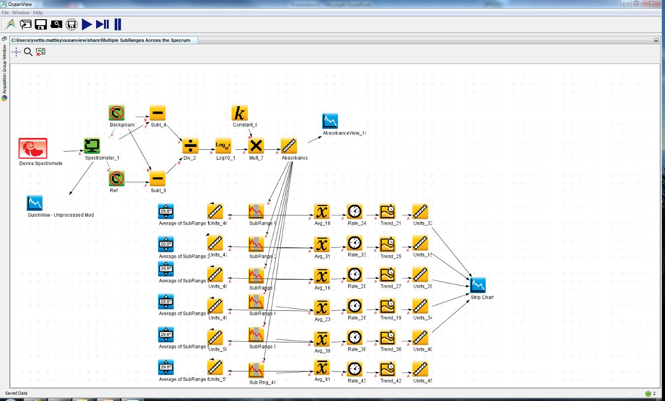
In this Schematic, we outline the process of measuring absorbance over subranges and then averaging Absorbance values over time.

   7. Calculate the average of each subrange and display it in a Scalar view.

    a) Right-click on an empty part of the Schematic and select Basic Math | Average to add an Average node to the Schematic.
    b) CTRL+click and drag from the Subrange node to the Average node to connect the nodes.
    c) Right-click on an empty part of the Schematic and select Constant | Unit Labels to add a Unit Labels node to the Schematic.
    d) Double-click the Unit Labels node to enter data labels for your Scalar View. Type “Average Absorbance from XXX – XXX nm” (replace the XXX’s with the starting and ending wavelengths for your subrange) in the Title Y Label box and “OD” in the Unit Y Label box or use your own data labels. Click Apply and then Exit to close the dialog box.
    e) CTRL+click and drag from the Average node to the Unit Labels node to connect the nodes.
    f) Right-click on an empty part of the Schematic and select View | Add Scalar View.
    g) Use CTRL+click and drag to connect the Unit Labels node to the Scalar node. The average of your subrange is now displayed in a Scalar view.
    h) Repeat steps 7a-7g to display the average of your other subranges in separate Scalar views.

8. Create a Strip Chart showing the change in your average Absorbance values over time.

    a) Click the Create Time Series Trend Chart button in the Scalar view to create a Strip Chart.
    b) Choose your Trend Update Rate. Select Update After Every Scan and Never Stop to plot every data point on your Strip Chart until you stop the acquisition. Click Finish.
    c) Repeat steps 8a-8b to create strip charts for the other subranges. Note that you can connect each of your Subranges to one Trend view to show all of the trends in one strip chart. Use a Unit Labels node to specify the axis labels.

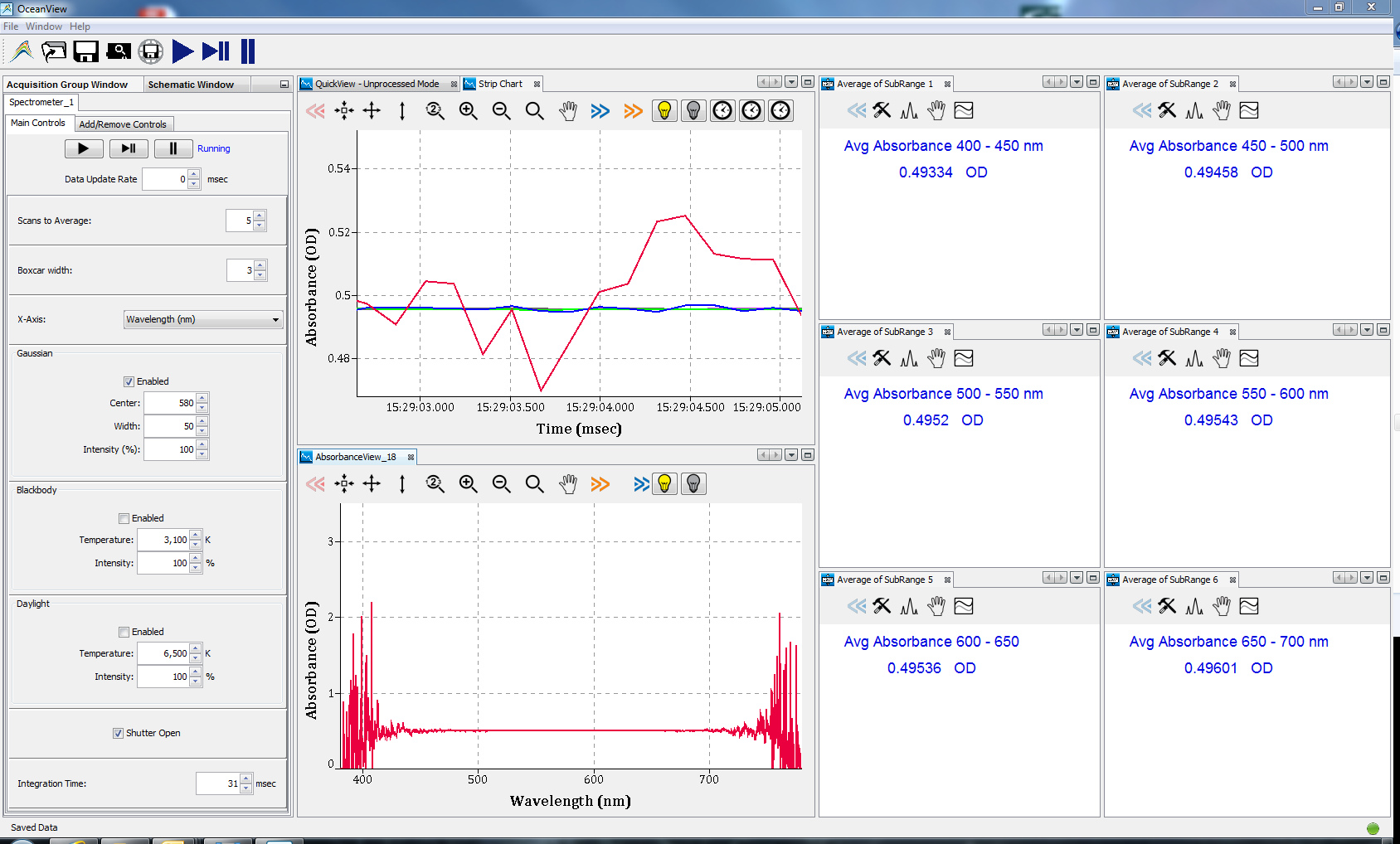With OceanView, you can calculate the average of subrange Absorbance values and show the change in values over time.